Download Series dc Circuits and more Study notes Law in PDF only on Docsity!
Series dc Circuits
5.1 INTRODUCTION
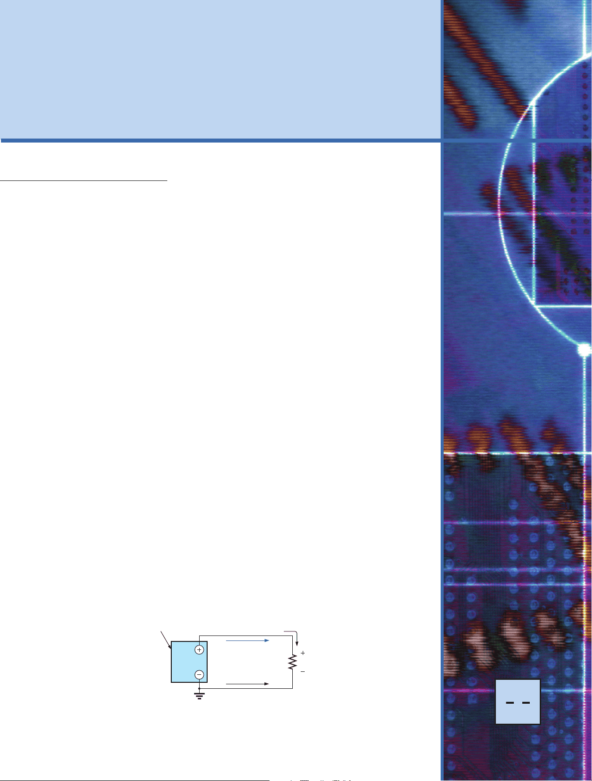
Two types of current are readily available to the consumer today. One is direct current (dc), in which ideally the flow of charge (current) does not change in magnitude (or direction) with time. The other is sinusoidal alternating current (ac), in which the flow of charge is continu- ally changing in magnitude (and direction) with time. The next few chapters are an introduc- tion to circuit analysis purely from a dc approach. The methods and concepts are discussed in detail for direct current; when possible, a short discussion suffices to cover any variations we may encounter when we consider ac in the later chapters. The battery in Fig. 5.1, by virtue of the potential difference between its terminals, has the ability to cause (or “pressure”) charge to flow through the simple circuit. The positive terminal attracts the electrons through the wire at the same rate at which electrons are supplied by the negative terminal. As long as the battery is connected in the circuit and maintains its terminal characteristics, the current (dc) through the circuit will not change in magnitude or direction. If we consider the wire to be an ideal conductor (that is, having no opposition to flow), the potential difference V across the resistor equals the applied voltage of the battery: V (volts) � E (volts).
- Become familiar with the characteristics of a series circuit and how to solve for the voltage, current, **_and power to each of the elements.
- Develop a clear understanding of Kirchhoff’s_** voltage law and how important it is to the analysis **_of electric circuits.
- Become aware of how an applied voltage will_** divide among series components and how to **_properly apply the voltage divider rule.
- Understand the use of single- and double-_** subscript notation to define the voltage levels of a **_network.
- Learn how to use a voltmeter, ammeter, and_** ohmmeter to measure the important quantities of a network.
S
Objectives
Series dc Circuits
Battery
E (volts)
I conventional
I electron
I = V R
E R = — R V
—
FIG. 5. Introducing the basic components of an electric circuit.
132 ⏐⏐⏐ SERIES dc CIRCUITS
For all one-voltage- source dc circuits
I^ E
FIG. 5. Defining the direction of conventional flow for single-source dc circuits.
I
V
R For any combination of voltage sources in the same dc circuit
FIG. 5. Defining the polarity resulting from a conventional current I through a resistive element.
a
b
R 1
10 �
R 2
30 �
R 3
100 � RT
FIG. 5. Series connection of resistors.
R 1
10 �
R 2
30 �
R 4 220 �
FIG. 5. Configuration in which none of the resistors are in series.
The current is limited only by the resistor R. The higher the resistance, the less the current, and conversely, as determined by Ohm’s law. By convention (as discussed in Chapter 2), the direction of conventional current flow ( I conventional) as shown in Fig. 5.1 is opposite to that of electron flow ( I electron). Also, the uniform flow of charge dictates that the direct current I be the same everywhere in the circuit. By following the direction of conventional flow, we notice that there is a rise in potential across the battery (� to �), and a drop in potential across the resistor (� to �). For single-voltage-source dc circuits, conventional flow always passes from a low potential to a high potential when passing through a volt- age source, as shown in Fig. 5.2. However, conventional flow always passes from a high to a low potential when passing through a resistor for any number of voltage sources in the same circuit, as shown in Fig. 5.3. The circuit in Fig. 5.1 is the simplest possible configuration. This chap- ter and the following chapters add elements to the system in a very specific manner to introduce a range of concepts that will form a major part of the foundation required to analyze the most complex system. Be aware that the laws, rules, and so on, introduced in Chapters 5 and 6 will be used through- out your studies of electrical, electronic, or computer systems. They are not replaced by a more advanced set as you progress to more sophisticated ma- terial. It is therefore critical that you understand the concepts thoroughly and are able to apply the various procedures and methods with confidence.
5.2 SERIES RESISTORS
Before the series connection is described, first recognize that every fixed resistor has only two terminals to connect in a configuration—it is there- fore referred to as a two-terminal device. In Fig. 5.4, one terminal of re- sistor R 2 is connected to resistor R 1 on one side, and the remaining terminal is connected to resistor R 3 on the other side, resulting in one, and only one, connection between adjoining resistors. When connected in this manner, the resistors have established a series connection. If three el- ements were connected to the same point, as shown in Fig. 5.5, there would not be a series connection between resistors R 1 and R 2. For resistors in series, the total resistance of a series configuration is the sum of the resistance levels. In equation form for any number ( N ) of resistors,
A result of Eq. (5.1) is that the more resistors we add in series, the greater the resistance, no matter what their value. Further, the largest resistor in a series combination will have the most impact on the total resistance. For the configuration in Fig. 5.4, the total resistance would be RT � R 1 � R 2 � R 3 � 10 � � 30 � � 100 � and RT � 140 �
RT � R 1 � R 2 � R 3 � R 4 �...^ � RN
134 ⏐⏐⏐ SERIES dc CIRCUITS
a
b
R 1
4.7 k�
R 3
2.2 k�
R 2
1 k�
R 5
1 k�
R 4 1 k� RT
FIG. 5. Series combination of resistors for Example 5.3.
RT
a
b
R 1
4.7 k�
R 2
1 k�
R 3
2.2 k�
R 5
1 k�
R 4 1 k�
FIG. 5. Series circuit of Fig. 5.9 redrawn to permit the use of Eq. (5.2): RT � NR.
RT
R 1 R 2 R 3
10 � 30 � 100 �
COM (^) +
200 Ω
FIG. 5. Using an ohmmeter to measure the total resistance of a series circuit.
EXAMPLE 5.3 Determine the total resistance for the series resistors (standard values) in Fig. 5.9. Solution: First, the order of the resistors is changed as shown in Fig. 5.10 to permit the use of Eq. (5.2). The total resistance is then RT � R 1 � R 3 � NR 2 � 4.7 k� � 2.2 k� � (3)(1 k�) � 9.9 k �
Analogies
Throughout the text, analogies are used to help explain some of the im- portant fundamental relationships in electrical circuits. An analogy is simply a combination of elements of a different type that are helpful in explaining a particular concept, relationship, or equation. Two analogies that work well for the series combination of elements are connecting different lengths of rope together to make the rope longer. Adjoining pieces of rope are connected at only one point, satisfying the definition of series elements. Connecting a third rope to the common point would mean that the sections of rope are no longer in a series. Another analogy is connecting hoses together to form a longer hose. Again, there is still only one connection point between adjoining sec- tions, resulting in a series connection.
Instrumentation
The total resistance of any configuration can be measured by simply con- necting an ohmmeter across the access terminals as shown in Fig. 5.11 for the circuit in Fig. 5.4. Since there is no polarity associated with resistance, either lead can be connected to point a, with the other lead connected to point b. Choose a scale that will exceed the total resistance of the circuit, and remember when you read the response on the meter, if a kilohm scale was selected, the result will be in kilohms. For Fig. 5.11, the 200 � scale of our chosen multimeter was used because the total resistance is 140 �. If the 2 k� scale of our meter were selected, the digital display would read 0.140, and you must recognize that the result is in kilohms. In the next section, another method for determining the total resis- tance of a circuit is introduced using Ohm’s law.
5.3 SERIES CIRCUITS
If we now take an 8.4 V dc supply and connect it in series with the series resistors in Fig. 5.4, we have the series circuit in Fig. 5.12.
SERIES CIRCUITS ⏐⏐⏐ 135
E 8.4 V
Is
RT
Is
10 �
V 1 R 1
100 �
V 3 R 3
30 �
V 2 Is R 2 Is Is
Is
FIG. 5. Schematic representation for a dc series circuit.
A circuit is any combination of elements that will result in a continuous flow of charge, or current, through the configuration.
First, recognize that the dc supply is also a two-terminal device with two points to be connected. If we simply ensure that there is only one connection made at each end of the supply to the series combination of resistors, we can be sure that we have established a series circuit. The manner in which the supply is connected determines the direction of the resulting conventional current. For series dc circuits:
the direction of conventional current in a series dc circuit is such that it leaves the positive terminal of the supply and returns to the negative terminal, as shown in Fig. 5.12.
One of the most important concepts to remember when analyzing se- ries circuits and defining elements that are in series is:
The current is the same at every point in a series circuit.
For the circuit in Fig. 5.12, the above statement dictates that the current is the same through the three resistors and the voltage source. In addition, if you are ever concerned about whether two elements are in series, sim- ply check whether the current is the same through each element.
In any configuration, if two elements are in series, the current must be the same. However, if the current is the same for two adjoining elements, the elements may or may not be in series.
The need for this constraint in the last sentence will be demonstrated in the chapters to follow. Now that we have a complete circuit and current has been established, the level of current and the voltage across each resistor should be deter- mined. To do this, return to Ohm’s law and replace the resistance in the equation by the total resistance of the circuit. That is,
with the subscript s used to indicate source current. It is important to realize that when a dc supply is connected, it does not “see” the individual connection of elements but simply the total re- sistance “seen” at the connection terminals, as shown in Fig. 5.13(a). In other words, it reduces the entire configuration to one such as in Fig. 5.13(b) to which Ohm’s law can easily be applied.
Is �
E
RT
SERIES CIRCUITS ⏐⏐⏐ 137
20 V R 2 1 �
R 1 = 2 �
V 1
V 2
R 3 = 5 �
V 3
E
Is
RT Is
FIG. 5. Series circuit to be investigated in Example 5.4.
Is R 1 = 7 �
RT Is
R 2 = 4 �
V 2
Is R^4
7 �
E 50 V^ R 3 7 �
FIG. 5. Series circuit to be analyzed in Example 5.5.
which for Fig. 5.12 results in
V 1 � I 1 R 1 � IsR 1 � (60 mA)(10 �) � 0.6 V V 2 � I 2 R 2 � IsR 2 � (60 mA)(30 �) � 1.8 V V 3 � I 3 R 3 � IsR 3 � (60 mA)(100 �) � 6.0 V Note that in all the numerical calculations appearing in the text thus far, a unit of measurement has been applied to each calculated quantity. Always remember that a quantity without a unit of measurement is often meaningless.
EXAMPLE 5.4 For the series circuit in Fig. 5.15:
a. Find the total resistance RT. b. Calculate the resulting source current Is. c. Determine the voltage across each resistor.
Solutions:
a. RT � R 1 � R 2 � R 3 � 2 � � 1 � � 5 � RT � 8 �
b.
c. V 1 � I 1 R 1 � IsR 1 � (2.5 A)(2 �) � 5 V V 2 � I 2 R 2 � IsR 2 � (2.5 A)(1 �) � 2.5 V V 3 � I 3 R 3 � IsR 3 � (2.5 A)(5 �) � 12.5 V
EXAMPLE 5.5 For the series circuit in Fig. 5.16:
a. Find the total resistance RT. b. Determine the source current Is and indicate its direction on the circuit. c. Find the voltage across resistor R 2 and indicate its polarity on the circuit.
Solutions:
a. The elements of the circuit are rearranged as shown in Fig. 5.17. RT � R 2 � NR � 4 � � (3)(7 �) � 4 � � 21 � RT � 25 �
Is �
E
RT
20 V
� 2.5 A
V 2
E = 50 V (^) R (^) T
Is
R 2
4 �
R 1
7 �
R 3
7 �
R 4
7 �
Is Is
Is
FIG. 5. Circuit in Fig. 5.16 redrawn to permit the use of Eq. (5.2).
138 ⏐⏐⏐ SERIES dc CIRCUITS
R 3 6 k�
R 2
E
RT = 12 k�
R 1
4 k�
I 3 = 6 mA
FIG. 5. Series circuit to be analyzed in Example 5.6.
b. Note that because of the manner in which the dc supply was con- nected, the current now has a counterclockwise direction as shown in Fig. 5.17.
c. The direction of the current will define the polarity for V 2 appearing in Fig. 5.17. V 2 � I 2 R 2 � IsR 2 � (2 A)(4 �) � 8 V
Examples 5.4 and 5.5 are straightforward, substitution-type problems that are relatively easy to solve with some practice. Example 5.6, how- ever, is another type of problem that requires both a firm grasp of the fun- damental laws and equations and an ability to identify which quantity should be determined first. The best preparation for this type of exercise is to work through as many problems of this kind as possible.
EXAMPLE 5.6 Given R (^) T and I 3, calculate R 1 and E for the circuit in Fig. 5.18. Solution: Since we are given the total resistance, it seems natural to first write the equation for the total resistance and then insert what we know. RT � R 1 � R 2 � R 3 We find that there is only one unknown, and it can be determined with some simple mathematical manipulations. That is, 12 k� � R 1 � 4 k� � 6 k� � R 1 � 10 k� and 12 k� � 10 k� � R 1 so that R 1 � 2 k � The dc voltage can be determined directly from Ohm’s law. E � IsRT � I 3 RT � (6 mA)(12 k�) � 72 V
Analogies
The analogies used earlier to define the series connection are also excel- lent for the current of a series circuit. For instance, for the series- connected ropes, the stress on each rope is the same as they try to hold the heavy weight. For the water analogy, the flow of water is the same through each section of hose as the water is carried to its destination.
Instrumentation
Another important concept to remember is: The insertion of any meter in a circuit will affect the circuit. You must use meters that minimize the impact on the response of the cir- cuit. The loading effects of meters are discussed in detail in a later sec- tion of this chapter. For now, we will assume that the meters are ideal and do not affect the networks to which they are applied so that we can con- centrate on their proper usage.
Is �
E
RT
50 V
� 2 A
140 ⏐⏐⏐ SERIES dc CIRCUITS
- 4 0
6 0. 0
V O L T A G E
C U R R E N T ( mA ) + (^) OFF ON
Coarse Fine Coarse Fine
CV
CC
mA COM +
200mA
R 1 R 2 R 3
I (^) s
+^ COM
+^ COM
+^ COM
I (^) s I (^) s Is I^ s
I (^) s
10 � 30 � 100 �
200mA mA 200mA mA 200mA mA
FIG. 5. Measuring the current throughout the series circuit in Fig. 5.12.
E
R 1 R 2 R 3
PE
P (^) R 1
P (^) R 2 PR 3
Is
FIG. 5. Power distribution in a series circuit.
negative terminal. This was done for three of the ammeters, with the am- meter to the right of R 3 connected in the reverse manner. The result is a negative sign for the current. However, also note that the current has the correct magnitude. Since the current is 60 mA, the 200 mA scale of our meter was used for each meter. As expected, the current at each point in the series circuit is the same using our ideal ammeters.
5.4 POWER DISTRIBUTION IN A SERIES CIRCUIT
In any electrical system, the power applied will equal the power dissi- pated or absorbed. For any series circuit, such as that in Fig. 5.21, the power applied by the dc supply must equal that dissipated by the resistive elements. In equation form,
PE � PR 1 � PR 2 � PR 3 (5.5)
VOLTAGE SOURCES IN SERIES ⏐⏐⏐ 141
R 3 2 k�
R 2
PR 1
E
R (^) T
R 1
36 V
3 k�
Is
1 k�
V 1 V 2
V 3
PE
PR 2
PR 3
FIG. 5. Series circuit to be investigated in Example 5.7.
The power delivered by the supply can be determined using
(watts, W) (5.6)
The power dissipated by the resistive elements can be determined by any of the following forms (shown for resistor R 1 only):
(watts, W) (5.7)
Since the current is the same through series elements, you will find in the following examples that
in a series configuration, maximum power is delivered to the largest resistor.
EXAMPLE 5.7 For the series circuit in Fig. 5.22 (all standard values):
a. Determine the total resistance RT. b. Calculate the current Is. c. Determine the voltage across each resistor. d. Find the power supplied by the battery. e. Determine the power dissipated by each resistor. f. Comment on whether the total power supplied equals the total power dissipated.
Solutions:
a. RT � R 1 � R 2 � R 3 � 1 k� � 3 k� � 2 k� RT � 6 k �
b.
c. V 1 � I 1 R 1 � Is R 1 � (6 mA)(1 k�) � 6 V V 2 � I 2 R 2 � Is R 2 � (6 mA)(3 k�) � 18 V V 3 � I 3 R 3 � Is R 3 � (6 mA)(2 k�) � 12 V d. PE � EI s � (36 V)(6 mA) � 216 mW e.
f. (checks)
5.5 VOLTAGE SOURCES IN SERIES
Voltage sources can be connected in series, as shown in Fig. 5.23, to in- crease or decrease the total voltage applied to a system. The net voltage is determined by summing the sources with the same polarity and sub- tracting the total of the sources with the opposite polarity. The net polar- ity is the polarity of the larger sum.
216 mW � 36 mW � 108 mW � 72 mW � 216 mW
PE � PR 1 � PR 2 � PR 3
P 3 �
V 32
R 3
1 12 V 22
2 k�
� 72 mW
P 2 � I^22 R 2 � 1 6 mA 221 3 k� 2 � 108 mW
P 1 � V 1 I 1 � 1 6 V2 16 mA 2 � 36 mW
Is �
E
RT
36 V
6 k�
� 6 mA
P 1 � V 1 I 1 � I 12 R 1 �
V 12
R 1
PE � EIs
KIRCHHOFF’S VOLTAGE LAW ⏐⏐⏐ 143
60 V
4 0. 0
- 0 0
V O L T A G E
C U R R E N T + (^) OFF ON
Coarse Fine Coarse Fine
CV
CC
2 0. 0
- 0 0
V O L T A G E
C U R R E N T + (^) OFF ON
Coarse Fine Coarse Fine
CV
CC
a
b
a
b
20 V
40 V
E 2
E 1
60 V
(c)
20 V
40 V
20 V?
E 2
E 1
0 V
0 V
a
b
Short across supply E 1 (b)
4 0. 0
- 0 0
V O L T A G E
C U R R E N T + (^) OFF ON
Coarse Fine Coarse Fine
CV
CC
2 0. 0
- 0 0
V O L T A G E
C U R R E N T + (^) OFF ON
Coarse Fine Coarse Fine
CV
CC
a
b
60 V?
(a)
1.5 V
1.5 V 1.5 V
1.5 V
6 V
E 2
E 1
FIG. 5. Series connection of dc supplies: (a) four 1.5 V batteries in series to establish a terminal voltage of 6 V; (b) incorrect connections for two series dc supplies; (c) correct connection of two series supplies to establish 60 V at the output terminals.
feature for the users, a series connection of supplies cannot be made. Be aware of this fact, because some educational institutions add an internal ground to the supplies as a protective feature even though the panel still displays the ground connection as an optional feature.
5.6 KIRCHHOFF’S VOLTAGE LAW
The law to be described in this section is one of the most important in this field. It has application not only to dc circuits but also to any type of signal—whether it be ac, digital, and so on. This law is far-reaching and can be very helpful in working out solutions to networks that sometimes leave us lost for a direction of investigation. The law, called Kirchhoff’s voltage law (KVL), was developed by Gustav Kirchhoff (Fig. 5.25) in the mid-1800s. It is a cornerstone of the entire field and, in fact, will never be outdated or replaced. The application of the law requires that we define a closed path of in- vestigation, permitting us to start at one point in the network, travel through the network, and find our way back to the original starting point. The path does not have to be circular, square, or any other defined shape; it must sim- ply provide a way to leave a point and get back to it without leaving the
FIG. 5. Gustav Robert Kirchhoff. Courtesy of the Smithsonian Institution, Photo No. 58,283. German (Königsberg, Berlin) (1824–87) , Physicist Professor of Physics, University of Heidelberg Although a contributor to a number of areas in the physics domain, he is best known for his work in the electrical area with his definition of the relationships between the currents and voltages of a network in
- Did extensive research with German chemist Robert Bunsen (developed the Bunsen burner ), re- sulting in the discovery of the important elements of cesium and rubidium.
144 ⏐⏐⏐ SERIES dc CIRCUITS
R 2
R 1
V 1
E^ V 2
a b
d c
I I
I
KVL
FIG. 5. Applying Kirchhoff’s voltage law to a series dc circuit.
network. In Fig. 5.26, if we leave point a and follow the current, we will end up at point b. Continuing, we can pass through points c and d and even- tually return through the voltage source to point a, our starting point. The path abcda is therefore a closed path, or closed loop. The law specifies that the algebraic sum of the potential rises and drops around a closed path (or closed loop) is zero. In symbolic form it can be written as
(Kirchhoff’s voltage law in symbolic form) (5.8)
where Σ represents summation, A the closed loop, and V the potential drops and rises. The term algebraic simply means paying attention to the signs that result in the equations as we add and subtract terms. The first question that often arises is, Which way should I go around the closed path? Should I always follow the direction of the current? To simplify matters, this text will always try to move in a clockwise direc- tion. By selecting a direction, you eliminate the need to think about which way would be more appropriate. Any direction will work as long as you get back to the starting point. Another question is, How do I apply a sign to the various voltages as I proceed in a clockwise direction? For a particular voltage, we will assign a positive sign when proceeding from the negative to positive potential— a positive experience such as moving from a negative checking balance to a positive one. The opposite change in potential level results in a negative sign. In Fig. 5.26, as we proceed from point d to point a across the voltage source, we move from a negative potential (the negative sign) to a positive potential (the positive sign), so a positive sign is given to the source voltage E. As we proceed from point a to point b, we encounter a positive sign fol- lowed by a negative sign, so a drop in potential has occurred, and a negative sign is applied. Continuing from b to c, we encounter another drop in po- tential, so another negative sign is applied. We then arrive back at the start- ing point d, and the resulting sum is set equal to zero as defined by Eq. (5.8). Writing out the sequence with the voltages and the signs results in the following: � E � V 1 � V 2 � 0 which can be rewritten as E � V 1 � V 2 The result is particularly interesting because it tells us that the applied voltage of a series dc circuit will equal the sum of the voltage drops of the circuit. Kirchhoff’s voltage law can also be written in the following form:
revealing that the sum of the voltage rises around a closed path will always equal the sum of the voltage drops. To demonstrate that the direction that you take around the loop has no effect on the results, let’s take the counterclockwise path and compare re- sults. The resulting sequence appears as
� E � V 2 � V 1 � 0 yielding the same result of E � V 1 � V 2
©A V rises � ©A V drops
©A V � 0
146 ⏐⏐⏐ SERIES dc CIRCUITS
40 V
60 V Vx
30 V
FIG. 5. Series configuration to be examined in Example 5.11.
6 V
2 V
14 V
Vx
a
b
FIG. 5. Applying Kirchhoff’s voltage law to a circuit in which the polarities have not been provided for one of the voltages (Example 5.12).
For path 2, starting at point a in a clockwise direction, � V 2 � 20 V � 0 and V 2 � � 20 V The minus sign in the solution simply indicates that the actual polari- ties are different from those assumed.
The next example demonstrates that you do not need to know what elements are inside a container when applying Kirchhoff’s voltage law. They could all be voltage sources or a mix of sources and resistors. It doesn’t matter—simply pay strict attention to the polarities encountered. Try to find the unknown quantities in the next examples without look- ing at the solutions. It will help define where you may be having trouble. Example 5.11 emphasizes the fact that when you are applying Kirch- hoff’s voltage law, the polarities of the voltage rise or drop are the im- portant parameters, not the type of element involved.
EXAMPLE 5.11 Using Kirchhoff’s voltage law, determine the un- known voltage for the circuit in Fig. 5.30. Solution: Note that in this circuit, there are various polarities across the unknown elements since they can contain any mixture of compo- nents. Applying Kirchhoff’s voltage law in the clockwise direction re- sults in �60 V � 40 V � Vx � 30 V � 0 and Vx � 60 V � 30 V � 40 V � 90 V � 40 V with Vx � 50 V
EXAMPLE 5.12 Determine the voltage Vx for the circuit in Fig. 5.31. Note that the polarity of Vx was not provided. Solution: For cases where the polarity is not included, simply make an assumption about the polarity, and apply Kirchhoff’s voltage law as be- fore. If the result has a positive sign, the assumed polarity was correct. If the result has a minus sign, the magnitude is correct, but the assumed polarity must be reversed. In this case, if we assume point a to be posi- tive and point b to be negative, an application of Kirchhoff’s voltage law in the clockwise direction results in �6 V � 14 V � Vx � 2 V � 0 and Vx � �20 V � 2 V so that Vx � � 18 V Since the result is negative, we know that point a should be negative and point b should be positive, but the magnitude of 18 V is correct.
EXAMPLE 5.13 For the series circuit in Fig. 5.32.
a. Determine V 2 using Kirchhoff’s voltage law. b. Determine current I 2. c. Find R 1 and R 3.
VOLTAGE DIVISION IN A SERIES CIRCUIT ⏐⏐⏐ 147
I 2
E 54 V R 2 7 � V 2
R 1
V 1 = 18 V
V 3 = 15 V
R 3
FIG. 5. Series configuration to be examined in Example 5.13.
Solution:
a. Applying Kirchhoff’s voltage law in the clockwise direction starting at the negative terminal of the supply results in � E � V 3 � V 2 � V 1 � 0 and E � V 1 � V 2 � V 3 (as expected) so that V 2 � E � V 1 � V 3 � 54 V � 18 V � 15 V and V 2 � 21 V
b.
I 2 � 3A
c.
with
EXAMPLE 5.14 Using Kirchhoff’s voltage law and Fig. 5.12, verify Eq. (5.1).
Solution: Applying Kirchhoff’s voltage law around the closed path:
E � V 1 � V 2 � V 3
Substituting Ohm’s law:
Is RT � I 1 R 1 � I 2 R 2 � I 3 R 3 but Is � I 1 � I 2 � I 3 so that Is RT � Is ( R 1 � R 2 � R 3 ) and RT � R 1 � R 2 � R 3
which is Eq. (5.1).
5.7 VOLTAGE DIVISION IN A SERIES CIRCUIT
The previous section demonstrated that the sum of the voltages across the resistors of a series circuit will always equal the applied voltage. It can- not be more or less than that value. The next question is, How will a re- sistor’s value affect the voltage across the resistor? It turns out that
the voltage across series resistive elements will divide as the magnitude of the resistance levels.
In other words,
in a series resistive circuit, the larger the resistance, the more of the applied voltage it will capture.
In addition,
the ratio of the voltages across series resistors will be the same as the ratio of their resistance levels.
All of the above statements can best be described by a few simple ex- amples. In Fig. 5.33, all the voltages across the resistive elements are pro- vided. The largest resistor of 6 � captures the bulk of the applied voltage, while the smallest resistor, R 3 , has the least. In addition, note that since the resistance level of R 1 is six times that of R 3 , the voltage across R 1 is six times that of R 3. The fact that the resistance level of R 2 is three times that of R 1
R 3 �
V 3
I 3
15 V
3 A
R 1 �
V 1
I 1
18 V
3 A
I 2 �
V 2
R 2
21 V
R 3 1 � 2 V
R 2 3 � 6 V
R 1 6 �12 V
E 20 V
FIG. 5. Revealing how the voltage will divide across series resistive elements.
VOLTAGE DIVISION IN A SERIES CIRCUIT ⏐⏐⏐ 149
of the circuit. The rule itself can be derived by analyzing the simple se- ries circuit in Fig. 5.36. First, determine the total resistance as follows: RT � R 1 � R 2
Then
Apply Ohm’s law to each resistor:
The resulting format for V 1 and V 2 is
(voltage divider rule) (5.10)
where V (^) x is the voltage across the resistor R (^) x , E is the impressed volt- age across the series elements, and R (^) T is the total resistance of the se- ries circuit. The voltage divider rule states that
the voltage across a resistor in a series circuit is equal to the value of that resistor times the total applied voltage divided by the total resistance of the series configuration.
Although Eq. (5.10) was derived using a series circuit of only two ele- ments, it can be used for series circuits with any number of series resistors.
EXAMPLE 5.15 For the series circuit in Fig. 5.37.
a. Without making any calculations, how much larger would you ex- pect the voltage across R 2 to be compared to that across R 1? b. Find the voltage V 1 using only the voltage divider rule. c. Using the conclusion of part (a), determine the voltage across R 2. d. Use the voltage divider rule to determine the voltage across R 2 , and compare your answer to your conclusion in part (c). e. How does the sum of V 1 and V 2 compare to the applied voltage?
Solutions:
a. Since resistor R 2 is three times R 1 , it is expected that V 2 � 3 V 1.
b.
c. V 2 � 3 V 1 � 3(16 V) � 48 V
d.
The results are an exact match. e. E � V 1 � V 2 64 V � 16 V � 48 V � 64 V (checks)
V 2 � R 2
E
RT
� 160 �2 a
64 V
b � 48 V
V 1 � R 1
E
RT
� 20 � a
64 V
b � 20 � a
64 V
b � 16 V
Vx � Rx
E
RT
V 2 � I 2 R 2 � a
E
RT
b R 2 � R 2
E
RT
V 1 � I 1 R 1 � a
E
RT
b R 1 � R 1
E
RT
Is � I 1 � I 2 �
E
RT
V 2
E
R 2
R 1 V 1
I
RT
FIG. 5. Developing the voltage divider rule.
64 V
R 2
60 �
R 1
20 �
E
V 1 V 2
FIG. 5. Series circuit to be examined using the voltage divider rule in Example 5.15.
150 ⏐⏐⏐ SERIES dc CIRCUITS
E 45 V (^) R 2 5 k�
R 1 2 k�^ V 1
R 3 8 k�^ V 3
V'
FIG. 5. Series circuit to be investigated in Examples 5. and 5.17.
20V
V COM +
R 1 4.7 k�
R 2 1.2 k�
R 3 3 k� V 3
R 4 10 k�
FIG. 5. Voltage divider action for Example 5.18.
EXAMPLE 5.16 Using the voltage divider rule, determine voltages V 1 and V 3 for the series circuit in Fig. 5.38. Solution:
and
The voltage divider rule can be extended to the voltage across two or more series elements if the resistance in the numerator of Eq. (5.10) is ex- panded to include the total resistance of the series resistors across which the voltage is to be found ( R �). That is,
EXAMPLE 5.17 Determine the voltage (denoted V �) across the series combination of resistors R 1 and R 2 in Fig. 5.38. Solution: Since the voltage desired is across both R 1 and R 2 , the sum of R 1 and R 2 will be substituted as R � in Eq. (5.11). The result is R � � R 1 � R 2 � 2 k� � 5 k� � 7 k�
and
In the next example you are presented with a problem of the other kind: Given the voltage division, you must determine the required resis- tor values. In most cases, problems of this kind simply require that you are able to use the basic equations introduced thus far in the text.
EXAMPLE 5.18 Given the voltmeter reading in Fig. 5.39, find voltage V 3. Solution: Even though the rest of the network is not shown and the cur- rent level has not been determined, the voltage divider rule can be applied by using the voltmeter reading as the full voltage across the series com- bination of resistors. That is,
EXAMPLE 5.19 Design the voltage divider circuit in Fig. 5.40 such that the voltage across R 1 will be four times the voltage across R 2 ; that is, VR 1 � 4 VR 2.
V 3 � 4 V
V 3 � R 3
1 V meter 2 R 3 � R 2
3 k� 1 5.6 V 2 3 k� � 1.2 k�
V � � R �
E
RT
� 7 k� a
45 V
15 k�
b � 21 V
V � � R �
E
RT
V 3 � R 3
E
RT
� 8 k� a
45 V
b � 24 V
V 1 � R 1
E
RT
� 2 k� a
45V
15k�
b � 6 V
RT � 15k�
� 2 k� � 5 k� � 8 k�
RT � R 1 � R 2 � R 3
E 20 V R 2
R 1^ VR 1
VR 2
4 mA
FIG. 5. Designing a voltage divider circuit (Example 5.19).