Sample Exam 3: Solutions
#1)
"!#%$'&)(*+-,%#%$'&.'&.+/02134
"567
!89$+&;:
<
,
9$'&.=
>14
"7
!#%$?&
:
@
,
9$+&A
8134
47
!3.$?&)
:
B=
,
81#4
"7
!#%$?&)
:
<0
/8CD
0E!#
(
+=0
0>CD
/ !8
(
@0>1#C
56F7
&
4G.@&AH
B=/81#C
567
&
GI'&
J
H
#+LKDMN8"O!#%$P+LKDMN8"O6%$P8?O8!#%$B/
JQRKDMN8O6#%$B/ KDMN84O86$SNT3U-4O6#%$VNAT3U-"O8"WX!83.$SD
Q KMN84O6X%$PY$PZ)W#!89$BDJ<
H
C
KDMN8O!#DJ@
H
C
G
G
H
BO
H
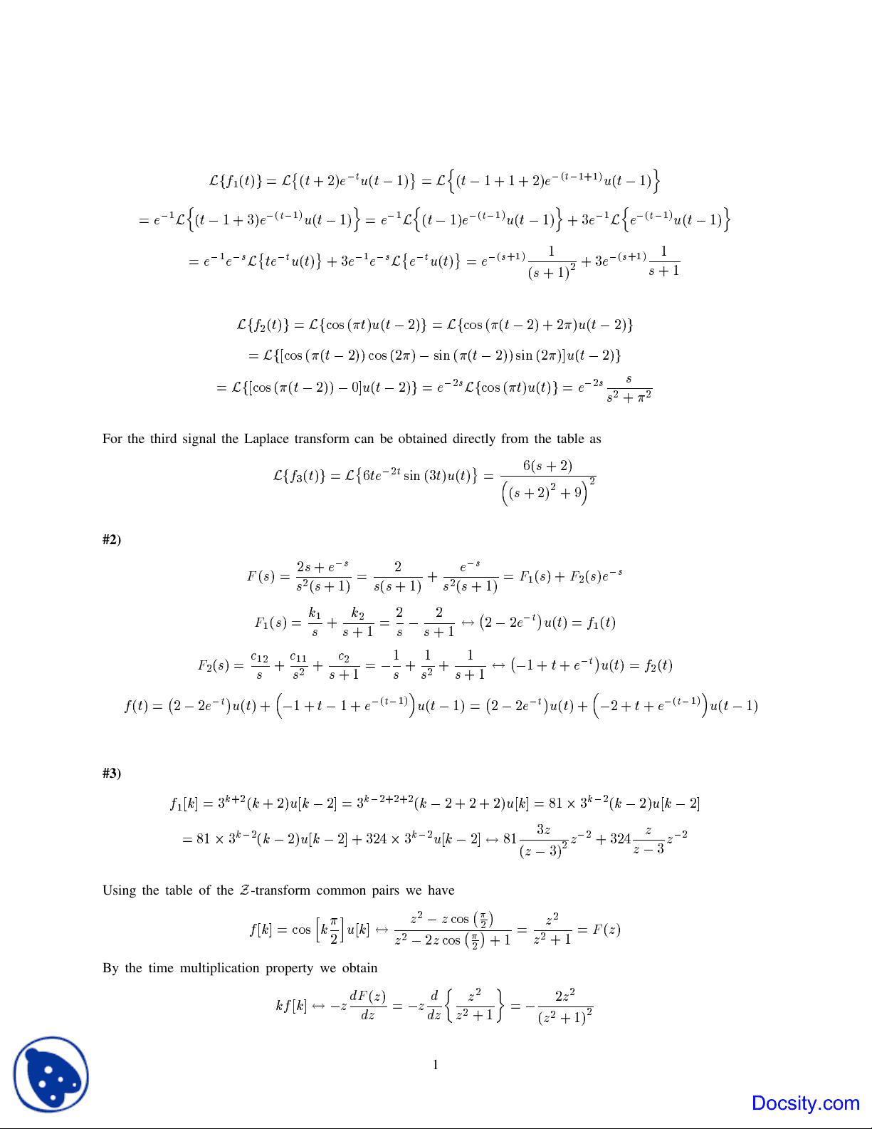
For the third signal the Laplace transform can be obtained directly from the table as
J/)[/DJ'
\
0
H
NAT]U-4=)A!8
(
\
"GIB
^
"GIB H+_)`
H
#2)
a
4Gb
Gc
8C
G
H
4G.@&
G/G.@&
8C
G
H
4G.@&
a
FG)8
a
H
"G)D/8C
a
4Gbed
G
d
H
G.@&
G
$
GI@&gfih
$S
E4j
!8.'
a
H
4G.lk
H
G
mk
D
G
H
k
H
GI'&
n$
&
G
&
G
H
&
G.@&gfih
$*&.V2?0E
j
!3.<
H
#
.
h
$P/ 4jL!#8
^
$*&co%$'&.B0>14
47
`!83.$+&.
h
$B0E4j/!#8
^
$JpV2?0>1q4
47
`!89$+&
#3)
Q
d
W>@=/r
5
H
d
+/D!2Q
d
$B;W>@=r0
H
5
H
5
H
d
$Bpp?/D!6Q
d
W8<s&Jtu=r0
H
d
$P!6Q
d
$S)W
'sv&-tu=r0
H
d
$P!6Q
d
$B)Ww+=)xytu=r0
H
!2Q
d
$B;W
f
sv&
=z
4z$B= H
z
H
?=/x
z
z$B=
z{
H
Using the table of the
|
-transform common pairs we have
6Q
d
W><KMN*}
d
O
%~
!6Q
d
W
f
z
H
$Bz.KDMN
hL
H
j
z
H
$Vz.KDMN
h
H
j
'&
z
H
z
H
@&
a
"z
By the time multiplication property we obtain
d
6Q
d
W
f
$Jz%
a
Xz
z
$Jz
zI
z
H
z
H
'&9
$
z
H
"z
H
'&) H
1
Docsity.com